Data Loading

I figured out how to load directly from the online csv.

library(dplyr)
library(ggplot2)
passwords <- readr::read_csv('https://raw.githubusercontent.com/rfordatascience/tidytuesday/master/data/2020/2020-01-14/passwords.csv')

## Parsed with column specification:
## cols(
##   rank = col_double(),
##   password = col_character(),
##   category = col_character(),
##   value = col_double(),
##   time_unit = col_character(),
##   offline_crack_sec = col_double(),
##   rank_alt = col_double(),
##   strength = col_double(),
##   font_size = col_double()
## )

passwords <- tbl_df(passwords)

glimpse(passwords)

## Observations: 507
## Variables: 9
## $ rank              <dbl> 1, 2, 3, 4, 5, 6, 7, 8, 9, 10, 11, 12, 13, 14, 15, …
## $ password          <chr> "password", "123456", "12345678", "1234", "qwerty",…
## $ category          <chr> "password-related", "simple-alphanumeric", "simple-…
## $ value             <dbl> 6.91, 18.52, 1.29, 11.11, 3.72, 1.85, 3.72, 6.91, 6…
## $ time_unit         <chr> "years", "minutes", "days", "seconds", "days", "min…
## $ offline_crack_sec <dbl> 2.170e+00, 1.110e-05, 1.110e-03, 1.110e-07, 3.210e-…
## $ rank_alt          <dbl> 1, 2, 3, 4, 5, 6, 7, 8, 9, 10, 11, 12, 13, 14, 15, …
## $ strength          <dbl> 8, 4, 4, 4, 8, 4, 8, 4, 7, 8, 8, 1, 32, 9, 9, 8, 8,…
## $ font_size         <dbl> 11, 8, 8, 8, 11, 8, 11, 8, 11, 11, 11, 4, 23, 12, 1…

Data Munging

The data variable types were already pretty well auto-classified but the category needed to be made into a factor.

passwords$category <- as.factor(passwords$category)

Exploration

I figured I would look at them by category. Here is the distribution by category. Some had NA category.

table(passwords$category, useNA = "ifany")

## 
##              animal          cool-macho              fluffy                food 
##                  29                  79                  44                  11 
##                name           nerdy-pop    password-related     rebellious-rude 
##                 183                  30                  15                  11 
## simple-alphanumeric               sport                <NA> 
##                  61                  37                   7

prop.table(table(passwords$category, useNA = "ifany"))

## 
##              animal          cool-macho              fluffy                food 
##          0.05719921          0.15581854          0.08678501          0.02169625 
##                name           nerdy-pop    password-related     rebellious-rude 
##          0.36094675          0.05917160          0.02958580          0.02169625 
## simple-alphanumeric               sport                <NA> 
##          0.12031558          0.07297830          0.01380671

passwords <- passwords %>% filter(!is.na(category))

Here’s how hard the passwords were to crack by category. They were all pretty easy to crack.

table(passwords$offline_crack_sec)

## 
## 1.11e-07 1.11e-06 4.75e-06 1.11e-05 0.000111 0.000124 0.000622  0.00111 
##       11        2       31       18        3       39        1        5 
##  0.00321   0.0111   0.0224   0.0835    0.806     2.17    29.02    29.27 
##      233        1        4       87        5       56        3        1

passwords %>% ggplot(aes(x = category, y = offline_crack_sec)) + 
  geom_boxplot() + scale_y_log10() + coord_flip()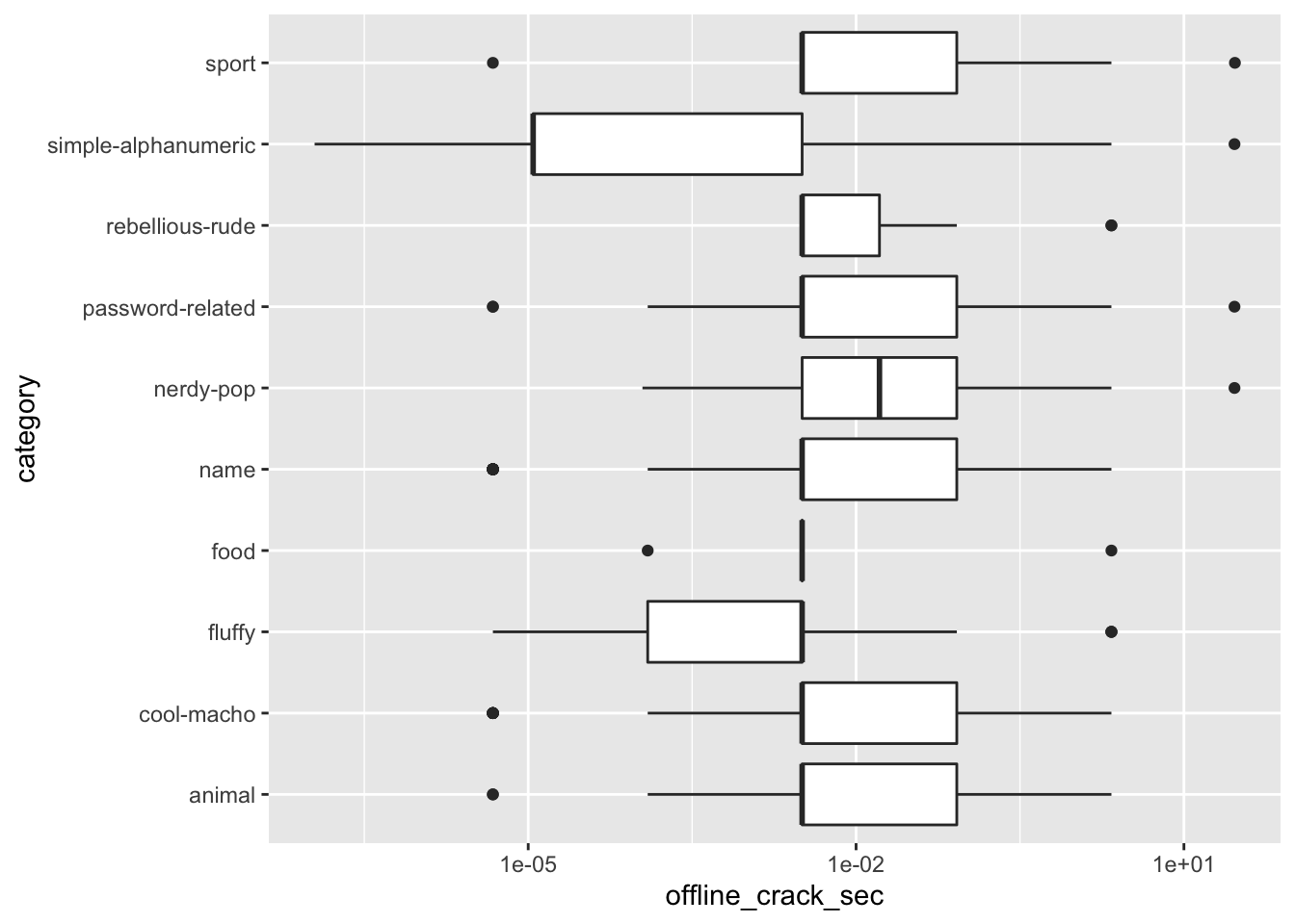

Popularity vs Difficulty to Crack

Was there a correlation between how popular they were and how easy they were to crack? Not clearly.

passwords %>% mutate(rank_crack = min_rank(offline_crack_sec)) %>%
  ggplot(aes(x = rank, y = rank_crack, color = category)) + 
  geom_point()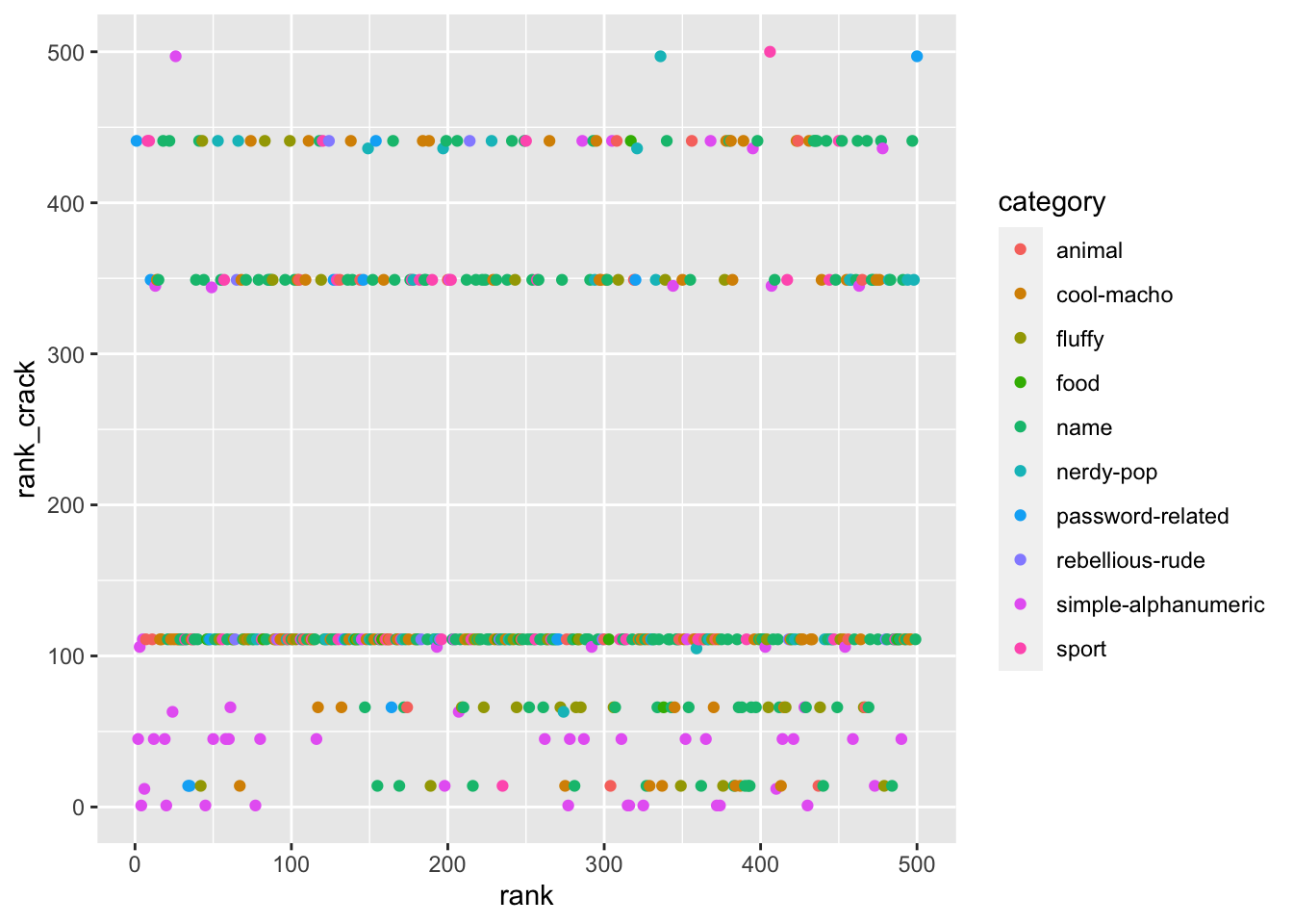

Conclusion

I couldn’t figure out much to do with this dataset but at least I got an idea of how to load a raw csv from Github.