Some more data fun with the Great Virtual Race across Tennessee. I decided I would like to look at how I’ve been doing in comparison to the other racers. I also added in the finishers (who are running back across Tennessee to Arkansas virtually).
One note about the data source for the finishers is that it is only complete from 5/1-5/17 for some reason. I suspect that this is because it’s about when the first finishers crossed the finish line. This might be problematic because it makes it hard to track their place among the other racers day by day between 5/17 and now. Because they are still ahead of me in cumulative mileage though, it doesn’t really matter for the ranks described below.
Data Loading and Cleaning
suppressPackageStartupMessages(library(tidyverse))
suppressPackageStartupMessages(library(lubridate))
gv <- read_csv("../datasets/gvrat_20200525.csv")## Parsed with column specification:
## cols(
## .default = col_double(),
## Position = col_character(),
## `Participant's Name` = col_character(),
## Event = col_character(),
## Home = col_character(),
## G = col_character(),
## KM = col_number(),
## `Your Approximate Location` = col_character(),
## `Comp%` = col_character(),
## `Proj Fin` = col_character()
## )## See spec(...) for full column specifications.bv <- read_csv("../datasets/gvbat_20200525.csv")## Parsed with column specification:
## cols(
## .default = col_double(),
## Position = col_character(),
## `Participant's Name` = col_character(),
## Event = col_character(),
## Home = col_character(),
## G = col_character(),
## `Your Approximate Location` = col_character(),
## `Comp%` = col_character(),
## `Proj Fin` = col_character()
## )
## See spec(...) for full column specifications.gv <- gv %>% filter(Event == "GVRAT")
# I got rid of the doggies running in the doggy virtual race
# Combine the finisher table and the active participant tables
gv <- bind_rows(gv, bv)
rm(bv)As last time I split the data into two tables: a roster and a miles run per day. This was because to use dplyr, you have to have it in long form, and the miles table didn’t need to have all that excess data from the roster on every long row.
gv_roster <- gv %>%
  select(Bib, name = `Participant's Name`, Event, G, A, Home, Miles) %>%
  mutate(Event = as.factor(Event)) %>%
  mutate(Home = as.factor(Home)) %>%
  mutate(G = as.factor(G))

gv_miles <- gv %>%
  select(-c(Position, `Participant's Name`, `Your Approximate   Location`,
            `Comp%`, `Proj Fin`, KM, Home, G, A, Miles)) %>%
  pivot_longer(contains("/"), names_to = "run_date", values_to = "miles_d") %>%
  mutate(run_date = mdy(paste0(run_date, "/2020"))) %>%
  mutate(Event = as.factor(Event))
My Average Distance Run
Here’s how far I have run or walked each day since signing up for the race on 5/13. Today (5/25) is not yet charted on the official table, so it is a 0 miles day so far.
gv_miles %>% filter(Bib == 18986) %>%
  ggplot(aes(x = run_date, y = miles_d)) +
  geom_bar(stat = "identity")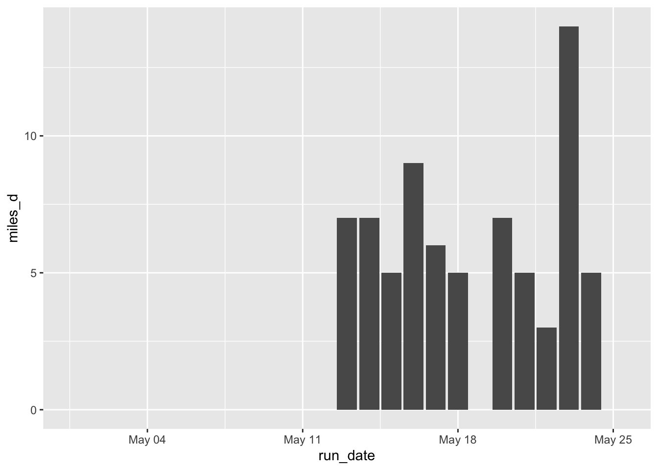
gv_miles %>% filter(Bib == 18986) %>%
  summarize(mean_miles = mean(miles_d), median_miles = median(miles_d))
## # A tibble: 1 x 2
## mean_miles median_miles
## <dbl> <dbl>
## 1 2.92 0Well I guess in May there were more days that I didn’t count versus days that did count. Let’s take out the days before May 13 and today May 25.
gv_miles %>% filter(Bib == 18986) %>%
  filter(run_date >= mdy("05-13-2020")) %>%
  filter(run_date < mdy("05-25-2020")) %>%
  summarize(mean_miles = mean(miles_d), median_miles = median(miles_d))
## # A tibble: 1 x 2
## mean_miles median_miles
## <dbl> <dbl>
## 1 6.08 5.5My Total Distance Run by Day
gv_miles %>% filter(Bib == 18986) %>%
  arrange(run_date) %>%
  mutate(miles_cumsum = cumsum(miles_d)) %>%
  filter(miles_d > 0)
## # A tibble: 11 x 5
## Bib Event run_date miles_d miles_cumsum
## <dbl> <fct> <date> <dbl> <dbl>
## 1 18986 GVRAT 2020-05-13 7 7
## 2 18986 GVRAT 2020-05-14 7 14
## 3 18986 GVRAT 2020-05-15 5 19
## 4 18986 GVRAT 2020-05-16 9 28
## 5 18986 GVRAT 2020-05-17 6 34
## 6 18986 GVRAT 2020-05-18 5 39
## 7 18986 GVRAT 2020-05-20 7 46
## 8 18986 GVRAT 2020-05-21 5 51
## 9 18986 GVRAT 2020-05-22 3 54
## 10 18986 GVRAT 2020-05-23 14 68
## 11 18986 GVRAT 2020-05-24 5 73My Position by Day
Calculating the position by day means figuring out the total miles per day then ranking everyone. That seems like it may become fairly calculation intensive, especially as the race moves along but it’s not too much for my humble laptop to handle right now.
gv_miles %>% group_by(Bib) %>%
  arrange(run_date) %>%
  mutate(miles_cumsum = cumsum(miles_d)) %>%
  ungroup() %>% group_by(run_date) %>%
  mutate(day_rank_absolute = min_rank(-miles_cumsum),
         percentile = percent_rank(miles_cumsum)) %>%
  filter(Bib == 18986, run_date >= mdy('05/12/2020')) %>%
  filter(run_date < today()) %>%
  select(run_date, miles_cumsum, day_rank_absolute, percentile)
## # A tibble: 13 x 4
## # Groups: run_date [13]
## run_date miles_cumsum day_rank_absolute percentile
## <date> <dbl> <int> <dbl>
## 1 2020-05-12 0 18253 0
## 2 2020-05-13 7 18075 0.0530
## 3 2020-05-14 14 17804 0.0657
## 4 2020-05-15 19 17597 0.0767
## 5 2020-05-16 28 17212 0.0967
## 6 2020-05-17 34 17009 0.107
## 7 2020-05-18 39 16839 0.115
## 8 2020-05-19 39 16947 0.109
## 9 2020-05-20 46 16685 0.123
## 10 2020-05-21 51 16559 0.129
## 11 2020-05-22 54 16521 0.131
## 12 2020-05-23 68 16011 0.158
## 13 2020-05-24 73 15880 0.165Just by starting running, I passed 5 percent of the entrants. Wow. One in twenty people paid $60 for this experience and haven’t run at all. So far, I’ve passed about 2500 runners!
Here’s the graphical representation
gv_miles %>% group_by(Bib) %>%
  arrange(run_date) %>%
  mutate(miles_cumsum = cumsum(miles_d)) %>%
  ungroup() %>% group_by(run_date) %>%
    mutate(percentile = percent_rank(miles_cumsum)) %>%
  filter(Bib == 18986) %>%
  ggplot(aes(x = run_date, y = percentile)) +
  geom_line()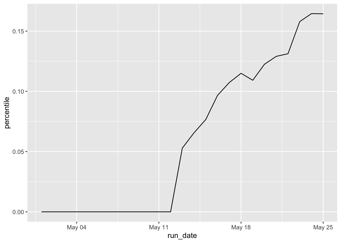
My Progress toward the Finish
There’s a couple of different ways of looking at my progress.
Progress vs. Buzzard
One way is looking at how I progress compared to the “Buzzard”. The Buzzard is the average distance required to be completed each day so that you can reach the finish line by the end of August. The rate is 634.84/122 or 5.204 miles per day. In the below figure I put the Buzzard as a red line.
gv_miles %>% filter(Bib == 18986) %>%
  arrange(run_date) %>%
  mutate(miles_cumsum = cumsum(miles_d)) %>%
  ggplot(aes(x = run_date, y = miles_cumsum)) +
  geom_line() +
  geom_abline(slope = 634.84/122,
              intercept = -634.84/122*(as.numeric(mdy("5/1/2020"))),
              color = "red") +
  scale_y_continuous(limits=c(0, 140)) +
  ylab("Total Miles Run") +
  xlab("Date")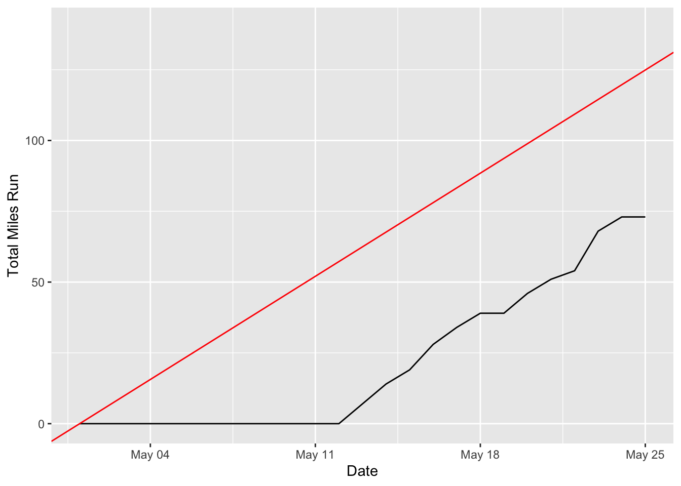
Projected Finish Date
To calculate the projected finish date I need my average miles per day. The race calculator starts the average from May 1.
gv_miles %>% filter(Bib == 18986) %>%
  arrange(run_date) %>%
  mutate(miles_cumsum = cumsum(miles_d), days = 1,
         days_cum = cumsum(days),
         days_remain = 122-days_cum) %>%
  mutate(ave_mileage = miles_cumsum/days_cum) %>%
  filter(ave_mileage > 0) %>%
  mutate(days_to_completion = 634.84/ave_mileage) %>%
  select(run_date, miles_cumsum, ave_mileage, days_to_completion, days_remain)
## # A tibble: 13 x 5
## run_date miles_cumsum ave_mileage days_to_completion days_remain
## <date> <dbl> <dbl> <dbl> <dbl>
## 1 2020-05-13 7 0.538 1179. 109
## 2 2020-05-14 14 1 635. 108
## 3 2020-05-15 19 1.27 501. 107
## 4 2020-05-16 28 1.75 363. 106
## 5 2020-05-17 34 2 317. 105
## 6 2020-05-18 39 2.17 293. 104
## 7 2020-05-19 39 2.05 309. 103
## 8 2020-05-20 46 2.3 276. 102
## 9 2020-05-21 51 2.43 261. 101
## 10 2020-05-22 54 2.45 259. 100
## 11 2020-05-23 68 2.96 215. 99
## 12 2020-05-24 73 3.04 209. 98
## 13 2020-05-25 73 2.92 217. 97The race director helpfully gives the projected finish date based on average miles.
gv_miles %>% filter(Bib == 18986) %>%
  arrange(run_date) %>%
  mutate(miles_cumsum = cumsum(miles_d), days = 1,
         days_cum = cumsum(days)) %>%
  mutate(ave_mileage = miles_cumsum/days_cum) %>%
  filter(miles_d > 0) %>%
  mutate(days_to_completion = 634.84/ave_mileage,
         projected_finish = days_to_completion + mdy("5/1/2020")) %>%
  select(run_date, miles_cumsum, days_to_completion, projected_finish)
## # A tibble: 11 x 4
## run_date miles_cumsum days_to_completion projected_finish
## <date> <dbl> <dbl> <date>
## 1 2020-05-13 7 1179. 2023-07-23
## 2 2020-05-14 14 635. 2022-01-25
## 3 2020-05-15 19 501. 2021-09-14
## 4 2020-05-16 28 363. 2021-04-28
## 5 2020-05-17 34 317. 2021-03-14
## 6 2020-05-18 39 293. 2021-02-18
## 7 2020-05-20 46 276. 2021-02-01
## 8 2020-05-21 51 261. 2021-01-17
## 9 2020-05-22 54 259. 2021-01-14
## 10 2020-05-23 68 215. 2020-12-01
## 11 2020-05-24 73 209. 2020-11-25I think I can do better if I use my actual average and add it to when I started on 5/13/2020.
gv_miles %>% filter(Bib == 18986) %>%
  arrange(run_date) %>%
  filter(run_date > mdy("5/12/2020")) %>%
  mutate(miles_cumsum = cumsum(miles_d), days = 1,
         days_cum = cumsum(days)) %>%
  mutate(ave_mileage = miles_cumsum/days_cum) %>%
  filter(miles_d > 0) %>%
  mutate(days_to_completion = 634.84/ave_mileage,
         projected_finish = days_to_completion + mdy("5/1/2020")) %>%
  select(run_date, miles_cumsum, days_to_completion, projected_finish)
## # A tibble: 11 x 4
## run_date miles_cumsum days_to_completion projected_finish
## <date> <dbl> <dbl> <date>
## 1 2020-05-13 7 90.7 2020-07-30
## 2 2020-05-14 14 90.7 2020-07-30
## 3 2020-05-15 19 100. 2020-08-09
## 4 2020-05-16 28 90.7 2020-07-30
## 5 2020-05-17 34 93.4 2020-08-02
## 6 2020-05-18 39 97.7 2020-08-06
## 7 2020-05-20 46 110. 2020-08-19
## 8 2020-05-21 51 112. 2020-08-21
## 9 2020-05-22 54 118. 2020-08-26
## 10 2020-05-23 68 103. 2020-08-11
## 11 2020-05-24 73 104. 2020-08-13Looks like I’m on track! Last week was a tapering week for the half marathon virtual race on Saturday so I only got in 39 miles including the race. That’s probably why the finish date got a little further out than when I first started.
I’m definitely planning on finishing on time but I want to pace myself this summer and let my body heal a bit. If I think about it my goal will be probably settle about 45 miles per week or 7 miles x 5 days and 10 miles on one longer day.