I’m almost at the end of May, and I’m over 100 miles into this race. It’s been a bit tough so far because of the time trial I did last week, but I’m still trying to get some cushion on the August 31 deadline for the race.
On the Facebook group for this race they talk about the races between races. Some people look at their state standings. Others may do their name rankings (i.e., rank among people named Smith or Mike).
I decided to look at how I’ve been doing compared to the other Hawaii runners and the runners with my first name. I also wanted to look at the people who have already finished and how they compare to the people who are still running.
Data Loading and Cleaning
suppressPackageStartupMessages(library(tidyverse))
suppressPackageStartupMessages(library(lubridate))
suppressPackageStartupMessages(library(scales))
suppressPackageStartupMessages(library(epiR))
gv <- read_csv("../datasets/gvrat_20200530.csv") # Active runners in GVRAT## Parsed with column specification:
## cols(
## .default = col_double(),
## Position = col_character(),
## `Participant's Name` = col_character(),
## Event = col_character(),
## Home = col_character(),
## G = col_character(),
## KM = col_number(),
## `Your Approximate Location` = col_character(),
## `Comp%` = col_character(),
## `Proj Fin` = col_character()
## )## See spec(...) for full column specifications.bv <- read_csv("../datasets/gvbat_20200530.csv") # Finshers who are going back## Parsed with column specification:
## cols(
## .default = col_double(),
## Position = col_character(),
## `Participant's Name` = col_character(),
## Event = col_character(),
## Home = col_character(),
## G = col_character(),
## KM = col_number(),
## `Your Approximate Location` = col_character(),
## `Comp%` = col_character(),
## `Proj Fin` = col_character()
## )
## See spec(...) for full column specifications.bv <- bv %>% mutate(finish = T)
gv <- gv %>% mutate(finish = F)
# Combine the finisher table and the active participant tables
gv <- bind_rows(gv, bv)
# I got rid of the doggies running in the doggy virtual race
gv <- gv %>% filter(Event == "GVRAT")
# Make data into long form for dplyr use
gv_miles <- gv %>%
select(-c(Position, `Participant's Name`, `Your Approximate Location`,
`Comp%`, `Proj Fin`, KM, Home, G, A, Miles)) %>%
pivot_longer(contains("/"), names_to = "run_date", values_to = "miles_d") %>%
mutate(run_date = mdy(paste0(run_date, "/2020"))) %>%
mutate(Event = as.factor(Event))
gv_roster <- gv %>%
select(Bib, name = `Participant's Name`, Event, G, A, Home, Miles, finish) %>%
mutate(Event = as.factor(Event)) %>%
mutate(Home = as.factor(Home)) %>%
mutate(G = as.factor(G))
rm(bv)
rm(gv)Hawaii Runners
There are now 42 runners from Hawaii.
Hawaii <- gv_roster %>% filter(Home == "USA - Hawaii") %>%
  mutate(place = dense_rank(-Miles)) %>%
  select(Bib, name, G, A, Miles, place)

Hawaii
## # A tibble: 42 x 6
## Bib name G A Miles place
## <dbl> <chr> <fct> <dbl> <dbl> <int>
## 1 9385 Duane Zitta M 39 398. 1
## 2 11868 Sally Cravens F 61 308. 2
## 3 17429 Aaron Reed M 28 296. 3
## 4 6786 April Shrum F 42 287 4
## 5 14940 G.M. Rumbaoa F 45 284. 5
## 6 6906 Robert Davidson M 37 273 6
## 7 7202 Chris Robinson M 39 244. 7
## 8 16629 michael hee M 60 243. 8
## 9 16019 Kana Yamamoto F 45 236. 9
## 10 13815 Andrew Borrebach M 29 229 10
## # … with 32 more rowsToday, I’m in place #31 among Hawaii runners.
These Hawaii people seem to be doing pretty good. No one is going crazy, with the clear leader having about 100 miles per week.
I decided to look at my rank compared to the other runners over time.
gv_miles %>% filter(Bib %in% Hawaii$Bib) %>%
  arrange(run_date) %>%
  group_by(Bib) %>%
  mutate(miles_t = cumsum(miles_d)) %>%
  ungroup %>%
  group_by(run_date) %>%
  mutate(place_d = min_rank(-miles_t)) %>%
  filter(Bib == 18986) %>%
  ggplot(aes(x = run_date, y = place_d)) + geom_line() +
  ylab("My place among Hawaii Runners") + xlab("Date")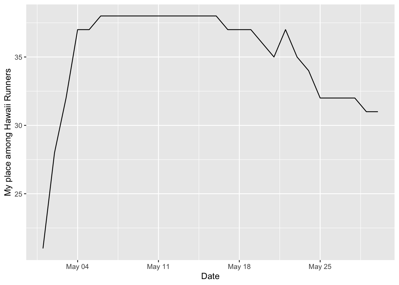
The Michaels
I could do the same thing for my name “Michael”.
Michael <- gv_roster %>% filter(grepl("Michael", name)) %>%
  mutate(place = dense_rank(-Miles)) %>%
  select(Bib, name, G, A, Miles, place)

Michael
## # A tibble: 220 x 6
## Bib name G A Miles place
## <dbl> <chr> <fct> <dbl> <dbl> <int>
## 1 54 Michael Maddock JR M 51 540. 1
## 2 1219 Michael O'Rourke M 44 489. 2
## 3 2690 Michael Scandrett M 39 422. 3
## 4 4027 Gary Michael M 65 417. 4
## 5 258 Michael Eriks M 36 388. 5
## 6 8543 Michael Miller M 49 386. 6
## 7 11678 Michael Small M 49 376. 7
## 8 5506 Michael Atcheson M 50 372. 8
## 9 10555 Michael Wells M 32 366. 9
## 10 13445 Michael Gampp M 51 337. 10
## # … with 210 more rowsThere are 220 Michaels in the race! Thanks in part to my late start I am in 160 place among Michaels.
Here are some other Michael characteristics.
Michael ages. Not too many young Michaels anymore since Michael hasn’t been as popular lately.
Michael %>% ggplot(aes(x = A)) +
  geom_histogram(binwidth = 5)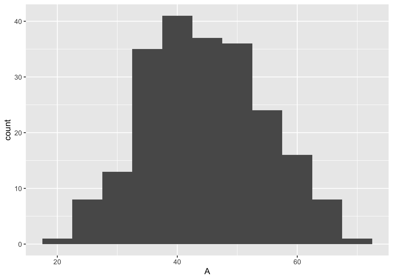
summary(Michael$A)## Min. 1st Qu. Median Mean 3rd Qu. Max.
## 19.00 37.00 44.00 44.41 51.00 69.00Michaels are doing great with their miles. If we were one giant commingled Michael who is running at the mean pace, we would be on track to finish the race.
summary(Michael$Miles)## Min. 1st Qu. Median Mean 3rd Qu. Max.
## 0.0 116.2 162.9 166.5 206.2 540.1Finisher Characteristics
Age and Gender for Finishers:
gv_roster %>% group_by(finish) %>%
  summarize(n(), mean_age = mean(A, na.rm = T),
            median_age = median(A, na.rm = T),
            male = mean(as.numeric(G)-1))
## # A tibble: 2 x 5
## finish `n()` mean_age median_age male
## <lgl> <int> <dbl> <dbl> <dbl>
## 1 FALSE 19090 43.8 44 0.435
## 2 TRUE 96 47.7 44 0.698So far, finishers are older than non-finishers and are more likely to be male.
Bivariate Comparisons
The 95% confidence interval of the difference in age is -6.9 to -0.8 years.
t.test(gv_roster$A ~ gv_roster$finish)##
## Welch Two Sample t-test
##
## data: gv_roster$A by gv_roster$finish
## t = -2.4831, df = 95.452, p-value = 0.01477
## alternative hypothesis: true difference in means is not equal to 0
## 95 percent confidence interval:
## -6.9218053 -0.7714575
## sample estimates:
## mean in group FALSE mean in group TRUE
## 43.80962 47.65625Now looking at the effect that gender has on finishing, we can see that females are about 1/3 as likely as males to have finished the race.
tab1 <- table(gv_roster$G, -gv_roster$finish)
tab1
##
## -1 0
## F 29 10792
## M 67 8298epi.2by2(tab1, method = "cross.sectional")## Warning in N0 * (N0 + N1) * a: NAs produced by integer overflow## Warning in N0 * N1 * (c + a): NAs produced by integer overflow
## Warning in N0 * N1 * (c + a): NAs produced by integer overflow## Warning in N0 * (N0 + N1) * a: NAs produced by integer overflow## Warning in N0 * N1 * (c + a): NAs produced by integer overflow
## Warning in N0 * N1 * (c + a): NAs produced by integer overflow## Outcome + Outcome - Total Prevalence * Odds
## Exposed + 29 10792 10821 0.268 0.00269
## Exposed - 67 8298 8365 0.801 0.00807
## Total 96 19090 19186 0.500 0.00503
##
## Point estimates and 95% CIs:
## -------------------------------------------------------------------
## Prevalence ratio 0.33 (0.22, 0.52)
## Odds ratio 0.33 (0.22, 0.51)
## Attrib prevalence * -0.53 (-0.75, -0.32)
## Attrib prevalence in population * -0.30 (-0.52, -0.09)
## Attrib fraction in exposed (%) -198.87 (-361.61, -93.50)
## Attrib fraction in population (%) -60.07 (-82.58, -40.35)
## -------------------------------------------------------------------
## Test that OR = 1: chi2(1) = 26.917 Pr>chi2 = <0.001
## Wald confidence limits
## CI: confidence interval
## * Outcomes per 100 population unitsrm(tab1)Putting both together, we can see that both age and gender are independently associated with finisher status.
model1 <- glm(finish ~ A + G, data = gv_roster, family = "binomial")
summary(model1)
##
## Call:
## glm(formula = finish ~ A + G, family = "binomial", data = gv_roster)
##
## Deviance Residuals:
## Min 1Q Median 3Q Max
## -0.2489 -0.1191 -0.0853 -0.0698 3.6177
##
## Coefficients:
## Estimate Std. Error z value Pr(>|z|)
## (Intercept) -7.315950 0.460805 -15.876 < 2e-16 ***
## A 0.030947 0.009018 3.432 6e-04 ***
## GM 1.071827 0.223077 4.805 1.55e-06 ***
## ---
## Signif. codes: 0 '***' 0.001 '**' 0.01 '*' 0.05 '.' 0.1 ' ' 1
##
## (Dispersion parameter for binomial family taken to be 1)
##
## Null deviance: 1208.6 on 19183 degrees of freedom
## Residual deviance: 1170.6 on 19181 degrees of freedom
## (2 observations deleted due to missingness)
## AIC: 1176.6
##
## Number of Fisher Scoring iterations: 8The odds of finishing for females were 1/3 those of males independent of age. Since the outcome is so rare (<1%) the odds ratio closely approximates the prevalence rate ratio.